B: Soft Matter, Fluid Interfaces, Colloids, Polymers, and Glassy MaterialsJanuary 20, 2026

Routes to the Density Profile and Structural Inconsistency
Click to copy article linkArticle link copied!

S. M. Tschopp*
S. M. Tschopp
Department of Physics, University of Fribourg, CH-1700 Fribourg, Switzerland
*Email: [email protected]
More by S. M. Tschopp
https://orcid.org/0000-0003-3259-052X
H. Vahid*
H. Vahid
Leibniz-Institute for Polymer Research, Institute Theory of Polymers, D-01069 Dresden, Germany
*Email: [email protected]
More by H. Vahid
J. M. Brader*
J. M. Brader
Department of Physics, University of Fribourg, CH-1700 Fribourg, Switzerland
*Email: [email protected]
More by J. M. Brader

Open PDF

The Journal of Physical Chemistry B

Cite this: J. Phys. Chem. B 2026, 130, 4, 1424–1436

Click to copy citationCitation copied!

https://doi.org/10.1021/acs.jpcb.5c07785

Published January 20, 2026

Request reuse permissions

Abstract

Click to copy section linkSection link copied!

Classical density functional theory (DFT) is the primary method for investigations of inhomogeneous fluids in external fields. It requires the excess Helmholtz free energy functional as input to an Euler–Lagrange equation for the one-body density. A variant of this methodology, the force-DFT, uses instead the Yvon–Born–Green equation to generate density profiles. It is known that the latter are consistent with the virial route to the thermodynamics, while DFT is consistent with the compressibility route. In this work we will show an alternative DFT scheme using the Lovett–Mou–Buff–Wertheim (LMBW) equation to obtain density profiles, that are shown to be also consistent with the compressibility route. However, force-DFT and LMBW DFT can both be implemented using a closure relation on the level of the two-body correlation functions. This is proven to be an advantageous feature, opening the possibility of an optimization scheme in which the structural inconsistency between different routes to the density profile is minimized. (“Structural inconsistency” is a generalization of the notion of thermodynamic inconsistency, familiar from bulk integral equation studies). Numerical results are given for the density profiles of two-dimensional systems of hard-core Yukawa particles with a repulsive or an attractive tail, in planar geometry.

This publication is licensed for personal use by The American Chemical Society.

Subjects

Special Issue

Published as part of The Journal of Physical Chemistry B special issue “Classical Density Functional Theory in Physical Chemistry”.

1. Introduction

Click to copy section linkSection link copied!

Density functional theory (DFT) provides an exact equilibrium framework for the study of classical many-body systems under the influence of external fields. The primary aim of DFT is to determine the one-body density profile and associated thermodynamic quantities by variational minimization of the grand potential functional. The nontrivial contribution to the grand potential is the excess (over ideal) Helmholtz free energy functional, F^exc, which encodes all information regarding the interparticle interactions and usually requires approximation.

For simple model systems with purely hard-core repulsive interactions the best known approximations to F^exc are given by fundamental measure theory (FMT). This approach has been shown to yield good results for many particle types of interest, such as spheres, (1−3) spherocylinders, (4) parallel cubes (5) and disks in two dimensions. (6) The situation is less satisfactory if the interaction potential is softly repulsive or has an attractive component (e.g., the Lennard-Jones potential). The former is usually dealt with by mapping onto an effective hard particle system, (7) whereas the latter are typically treated using either the simplest mean-field approximation (8,9) or other perturbative approaches. (10−12)

Given the challenges of directly approximating the free energy functional, it is not surprising that machine-learning (ML) methods are nowadays being exploited to either learn the free energy functional (13) or directly establish the connection between the one-body density and the direct correlation function (14,15)─the latter being the quantity required as input to the Euler–Lagrange (EL) equation for the density profile. Applications to specific systems, such as charged (16) or patchy (17,18) particles have proven quite successful. (For further details on machine learning in DFT we direct the reader to the recent review of Simon and Oettel. (19)) While ML approaches can be effective for interpolating and extrapolating simulation data they retain a certain “black box” character which does not reveal to the user the fundamental mechanisms at work in the many-body system. Consequently the desire to have a first-principles density functional scheme still remains.

It could be argued that the requirement of finding explicit analytic forms for F^exc is, in fact, overly demanding and that this has limited the range of systems which can be addressed using standard DFT methodology. An alternative scheme, which relaxes this restriction, is provided by the integral equation theory of inhomogeneous liquids. (20) Recent work has revived and reinterpreted the inhomogeneous integral equation approach in a way which makes clear that this is indeed a DFT, but formulated on the level of two-body functionals. (21) This theory represents a natural generalization of previous work on bulk fluids. If one looks back into the development of liquid-state theory, from Kirkwood to the present day, then the majority of approaches were focused on bulk systems for which the pair correlation functions played a central role. Knowledge of these provides both detailed information about the internal microstructure of the fluid and, in the case of pair interactions, enables the calculation of all thermodynamic properties. There is no reason to suppose that the two-body correlations are less important for inhomogeneous systems and it seems that the only reason for their underuse is the computational complexity of their calculation.

Let us first consider the bulk pair correlations. Thermodynamic quantities can be obtained from these via different routes, namely the compressibility and the virial. If the pair correlation functions are known exactly, then both routes are fully equivalent and yield identical results. However, since this is never the case for realistic model fluids, approximations are required, usually in the form of closures to the Ornstein–Zernike (OZ) integral equation. (22,23) Predictions for thermodynamic quantities, such as the pressure, then become dependent on the chosen route; a phenomenon referred to as thermodynamic inconsistency. (24−26)

Fortunately, thermodynamic inconsistency can be turned to our advantage by using it as a tool to generate improved approximation schemes. The development of thermodynamically consistent closures essentially began in 1973 with Waisman’s generalized mean-spherical approximation, in which a free parameter in the closure relation was determined by enforcing an accurate equation of state; (27) an idea further developed by Stell and Høye in ref (28). Subsequent focus was placed on the numerical determination of adjustable closure parameters to ensure consistency between the routes without imposing an equation of state as additional input to the theory. After the development of some classic consistent approximation schemes between 1979 and 1986, (29−33) the mid 1990s saw a resurgence of interest. (34−46) More recent attempts have largely been extensions/modifications of existing approximations to further improve accuracy, see e.g. refs (47–49).

Turning now to inhomogeneous fluids we observe that there exist two independent expressions relating the inhomogeneous two-body correlation functions to the one-body density, namely the Yvon–Born–Green (YBG) and the Lovett–Mou–Buff–Wertheim (LMBW) sum-rules. (50−58) The YBG equation has been used by the present authors to study confined fluids in two-dimensions, (21) but remains a relatively underexploited equation in studies of inhomogeneous fluids since its implementation presents certain technical challenges. In contrast, the LMBW equation is easier to numerically implement and has thus received more attention. Some examples are the studies by Omelyan et al. for the liquid–vapor interface, (59) by Brader for prefreezing phenomena (60) and by Nygå rd et al. for the prediction of local ordering in confined fluids. (61,62) Other works of interest are the study of hard-sphere solutes by Attard (63,64) and the investigation of systems under planar confinement by Kjellander and Sarman. (65)

The YBG and LMBW expressions are formally equivalent, they however generally yield different one-body density profiles if approximate two-body correlation functions are used as input. This sensitivity to the choice of sum-rule, which has recently been termed “structural inconsistency”, (21) adds a layer of complexity and sublety to the study of inhomogeneous integral equations which has so far received very little attention. Some clarity was gained in reference, (66) in which it was shown that the one-body density profiles obtained using the YBG equation are consistent with the virial route to the bulk thermodynamics. (This confirmed some earlier and long overlooked observations by Henderson (20)). The situation may be less clear for the case of the LMBW equation in which the one-body density is generated by integrating over the two-body direct correlation function.

In this paper we develop a LMBW DFT scheme. We test the contact theorem, which relates the bulk pressure to an integral over the inhomogeneous density profile. This reveals that the LMBW DFT generates compressibility consistent profiles. Standard DFT also yields compressibility consistent outcomes but, as already mentioned, always requires an expression for F^exc as input. In contrast, both the YBG and the LMBW DFT schemes are implementable using a closure relation. Since the YBG scheme yields virial results, we choose a closure relation involving a tuning parameter and vary it to enforce structural consistency between the two routes. We show numerical results, in two-dimensional planar geometry, for hard-core Yukawa particles with a repulsive or an attractive tail.

2. Methods

Click to copy section linkSection link copied!

2.1. Bulk Fluids

2.1.1. The Bulk Ornstein–Zernike Equation

In bulk the two-body correlation functions are solely dependent on the distance between two particle centers, r₁₂ ≡ |r₁ – r₂|. The total correlation function, h, and the two-body direct correlation, c, are linked via the bulk OZ equation (22,23)

h (r_{12}) = c (r_{12}) + ρ_{b} \int d r_{3} h (r_{13}) c (r_{32})

(1)

where ρ_b is the bulk density. The radial distribution function, g, is related to h according to g ≡ h + 1. Here and henceforth both volume integrals and densities have to be interpreted according to the spatial dimensionality under consideration. A supplementary closure relation between h and c is required to obtain a closed system of equations.

2.1.2. Two Routes to Calculate the Pressure

If the exact two-body correlations are employed, then each of the different routes to calculate the thermodynamical quantities yields fully consistent results and the choice of one over the other is purely a matter of computational convenience. However, if the two-body correlations are only known approximately, as is almost always the case, then the predictions from a given closure will vary from one choice of route to another.

2.1.2.1. The Virial Route

For a system in D dimensions interacting via a pairwise additive potential, ϕ, the virial pressure is given by

\frac{β P_{v}}{ρ_{b}} = 1 - \frac{β ρ_{b}}{2 D} \int d r r g (r) \frac{d ϕ (r)}{d r}

(2)

where

β \equiv {(k_{B} T)}^{- 1}

. This result can be derived straightforwardly from the Clausius virial. (22) For the two-dimensional systems to be addressed in the present work, eq 2 yields

\frac{β P_{v}}{ρ_{b}} \overset{2 D}{=} 1 - \frac{β ρ_{b}}{2} \int_{0}^{\infty} d r r^{2} g (r) \frac{d ϕ (r)}{d r}

(3)

We note that if ϕ has a discontinuity (e.g., for hard-core potentials), then one should be careful not to neglect the delta-function which occurs in its derivative. The virial expression 2 has the appealing feature that the pressure can be evaluated directly by spatial integration of the radial distribution function and does not require an integration over thermodynamic parameters.

2.1.2.2. The Compressibility Route

The isothermal compressibility, χ_T, is defined by the standard thermodynamic relation

χ_{T} = \frac{1}{ρ_{b}} {(\frac{\partial ρ_{b}}{\partial P})}_{T}

(4)

Alternatively, this can be expressed as an integral over the direct correlation function according to (22)

\frac{ρ_{b} χ_{T}}{β} = {(1 - ρ_{b} \int d r c (r))}^{- 1}

(5)

Unlike the virial equation, this expression does not rely on the assumption of pairwise additivity of the interparticle potential. Introducing the static structure factor, S, provides the following equivalent, but more compact, expression

\frac{ρ_{b} χ_{T}}{β} = {(1 - ρ_{b} \tilde{c} (k = 0))}^{- 1} \equiv S (k = 0)

(6)

where the tilde signifies a D-dimensional Fourier transform and k is the magnitude of the wavevector. Combining eqs 4 and 6 and integrating over the bulk density generates the familiar form for the compressibility pressure

\frac{β P_{c}}{ρ_{b}} = 1 - \frac{1}{ρ_{b}} \int_{0}^{ρ_{b}} d ρ ρ \tilde{c} (k = 0; ρ)

(7)

where the dependence of the correlation functions on the density has been made explicit in the notation.

We observe that implementation of eq 7 is problematic for systems exhibiting a liquid–gas phase transition arising from a mutual attraction between the particles. At low temperatures the integration path to values of ρ_b within the liquid phase will necessarily cross the spinodal region, where the direct correlation function appearing in eq 7 is not well-defined. The compressibility pressure at subcritical liquid states is thus not accessible, which then hinders the determination of a binodal.

2.2. Inhomogeneous Fluids

2.2.1. The Inhomogeneous Ornstein–Zernike Equation

When an external potential, V_ext, is applied to the system then the symmetry of the bulk is broken. This leads to a spatially varying one-body density, ρ(r), and to two-body correlations which in general depend on two vector positions. The two-body direct correlation function and total correlation function are now related to each other by the inhomogeneous OZ equation (9)

h (r_{1}, r_{2}) = c (r_{1}, r_{2}) + \int d r_{3} h (r_{1}, r_{3}) ρ (r_{3}) c (r_{3}, r_{2})

(8)

which recovers eq 1 in the bulk limit. In order to provide a closed framework for predictive calculation, eq 8 must be supplemented by (i) a closure relation between c and h containing details of the interparticle interaction and (ii) an exact sum-rule relating the inhomogeneous two-body correlations to the one-body density. Before considering approximate closures we will address the second point and discuss two distinct sum-rules (“routes”) for the one-body density.

2.2.2. Two Routes to the One-Body Density

The equilibrium one-body density is defined by the following grand canonical average (22)

ρ (r_{1}) = \frac{1}{Ξ} \sum_{N = 1}^{\infty} \frac{e^{β μ N}}{(N - 1)!} \int d r_{2} \cdot \cdot \cdot \int d r_{N} e^{- β U_{N}}

(9)

where Ξ is the grand canonical partition function, μ is the chemical potential and U_N is the total potential energy. For systems interacting via pairwise additive potentials the latter is given by

U_{N} ({r^{N}}) = \sum_{i = 1}^{N} V_{e x t} (r_{i}) + \frac{1}{2} \sum_{\begin{array}{l} i, j = 1 \\ i \neq j \end{array}}^{N} ϕ (r_{i j})

(10)

The inhomogeneous two-body density is defined by

ρ^{(2)} (r_{1}, r_{2}) = \frac{1}{Ξ} \sum_{N = 2}^{\infty} \frac{e^{β μ N}}{(N - 2)!} \int d r_{3} \cdot \cdot \cdot \int d r_{N} e^{- β U_{N}}

(11)

Both the one- and two-body densites are explicitly functionals of the external potential. Taking the functional derivative of eq 9 generates the first Yvon equation (8,67)

\frac{δ ρ (r_{1})}{δ β V_{e x t} (r_{2})} = - ρ (r_{1}) ρ (r_{2}) h (r_{1}, r_{2}) - ρ (r_{2}) δ (r_{1} - r_{2})

(12)

where the total correlation function is related to the two-body density according to

h (r_{1}, r_{2}) = \frac{ρ^{(2)} (r_{1}, r_{2})}{ρ (r_{1}) ρ (r_{2})} - 1

(13)

Since the one-body density and the external potential must satisfy the following functional chain-rule identity

\int d r_{3} \frac{δ ρ (r_{1})}{δ V_{e x t} (r_{3})} \frac{δ V_{e x t} (r_{3})}{δ ρ (r_{2})} = δ (r_{1} - r_{2})

(14)

and, since we have already stated eqs 8 and 12, it follows that the inverse of the latter must be given by

\frac{δ β V_{e x t} (r_{1})}{δ ρ (r_{2})} = c (r_{1}, r_{2}) - \frac{1}{ρ (r_{1})} δ (r_{1} - r_{2})

(15)

which is known as the second Yvon equation. (8,67) Note that eq 15 essentially defines the inhomogeneous two-body direct correlation function. (8,9,50)

2.2.2.1. The Yvon–Born–Green Equation

Taking the gradient of the one-body density 9 generates

\begin{array}{l} \nabla_{r_{1}} ρ (r_{1}) = - ρ (r_{1}) \nabla_{r_{1}} β V_{e x t} (r_{1}) \\ - \frac{β}{Ξ} \sum_{N = 2}^{\infty} \frac{e^{β μ N}}{(N - 2)!} \int d r_{2} \nabla_{r_{1}} ϕ (r_{12}) \int d r_{3} \cdot\cdot\cdot \int d r_{N} e^{- β U_{N}} \end{array}

(16)

Substituting the definition of the two-body density 11 into expression 16 then yields the first YBG equation

\begin{array}{l} \nabla_{r_{1}} ρ (r_{1}) = - ρ (r_{1}) \nabla_{r_{1}} β V_{e x t} (r_{1}) \\ - \int d r_{2} ρ^{(2)} (r_{1}, r_{2}) \nabla_{r_{1}} β ϕ (r_{12}) \end{array}

(17)

This sum-rule was derived long ago by Yvon (53) and Born and Green (54) and is a fundamental relation in statistical physics. Although we show here the standard derivation of eq 17 we note that an instructive alternative derivation can be found in ref (58). The YBG equation expresses the equilibrium force-balance between Brownian, external and internal forces, where the latter are intuitively expressed as a statistical average of the pair interaction force acting at the point r₁. The closed framework generated by the YBG eq 17, the inhomogeneous OZ eq 8 and an additional closure relation forms the force-DFT approach, (21,66) which provides an alternative to the standard (variational) implementation of classical DFT. (9,68)

2.2.2.2. The Lovett–Mou–Buff–Wertheim Equation

Taylor expanding the external potential about the point r₁ generates the following expression

\begin{array}{l} V_{e x t} (r_{1} + r^{'}) - V_{e x t} (r_{1}) \\ = \int d r_{2} \frac{δ V_{e x t} (r_{1})}{δ ρ (r_{2} + r^{'})} (ρ (r_{2} + r^{'}) - ρ (r_{2})) \end{array}

(18)

If the points r₁ and r′ lie close together, such that dr′ = r₁ – r′ is small in magnitude, then we can rewrite eq 18 using gradients, yielding

\nabla_{r_{1}} V_{e x t} (r_{1}) = \int d r_{2} \frac{δ V_{e x t} (r_{1})}{δ ρ (r_{2})} \nabla_{r_{2}} ρ (r_{2})

(19)

Substitution of the second Yvon eq 15 into expression 19 then leads to the LMBW equation (55,56)

\begin{array}{l} \nabla_{r_{1}} ρ (r_{1}) = - ρ (r_{1}) \nabla_{r_{1}} β V_{e x t} (r_{1}) \\ + ρ (r_{1}) \int d r_{2} c (r_{1}, r_{2}) \nabla_{r_{2}} ρ (r_{2}) \end{array}

(20)

For further insights we direct the reader to the papers of Lovett and Buff (57) and Baus and Lovett (58) as well as the excellent book by Widom and Rowlinson. (50)

2.2.3. Closure Relation Approximations

Using the indirect correlation function, γ ≡ h – c, the Verlet (V) and the Modified Verlet (MV) closure relations (25,30) impose that c(r₁, r₂) is given by

\overset{V}{=} e^{- β ϕ (r_{12}) + γ (r_{1}, r_{2}) - \frac{1}{2} γ^{2} (r_{1}, r_{2}) / 1 + \frac{4}{5} γ (r_{1}, r_{2})} - γ (r_{1}, r_{2}) - 1

(21)

\overset{M V}{=} e^{- β ϕ (r_{12}) + γ (r_{1}, r_{2}) - \frac{1}{2} γ^{2} (r_{1}, r_{2}) / 1 + α_{V} γ (r_{1}, r_{2})} - γ (r_{1}, r_{2}) - 1

(22)

respectively. The tuning parameter α_V in 22 is zero for γ < 0. The Verlet closure is known to perform very well not only in bulk systems, (25) but also in the inhomogeneous case. Indeed, in the recent paper, (21) the Verlet closure was tested against other closure relations, namely the Hypernetted chain, the Percus–Yevick and the Martinov–Sarkisov ones, for two-dimensional inhomogeneous fluids and proved very successful. In the present work we will thus use the Verlet closure in both original and modified versions.

2.2.4. Wall Contact Theorem

Let us consider a two-dimensional planar wall represented by the external potential V_ext(z), with the z-axes taken perpendicular to the wall. Since the one-body density always exhibits the same symmetry as the external potential, (8) it reduces to ρ(r) = ρ(z). For a generic wall potential, the following expression

β P = - \int_{- \infty}^{+ \infty} d z ρ (z) (\frac{d β V_{e x t} (z)}{d z})

(23)

holds. This is the general form of the so-called wall contact theorem that relates the bulk pressure, P, to the forces acting on the wall, making a link between the bulk equations of state discussed in Subsection 2.1.2 and the sum-rules for the inhomogeneous one-body density of Subsection 2.2.2.

For an external potential consisting of a hard wall plus an either repulsive or attractive tail, V_ext^tail(z), the derivative appearing in eq 23 picks up a delta-function contribution. In this case, the contact theorem is expressed as

β P = ρ (z_{w}) - \int_{z_{w}}^{+ \infty} d z ρ (z) (\frac{d β V_{e x t}^{t a i l} (z)}{d z})

(24)

where z_w is the z-coordinate of a particle in contact with the (hard) wall. (51)

2.3. Numerical Implementation

2.3.1. System of Interest: Specification of the Interparticle and External Potentials

2.3.1.1. Choice of the Interparticle Pair Potential

In this work we will consider a two-dimensional system of hard-core Yukawa (HCY) particles, given by the following pair potential

ϕ (r_{12}) = {\begin{array}{l} \infty, & r_{12} < d \\ κ \frac{e^{- α (r_{12} - d)}}{r_{12}}, & r_{12} \geq d \end{array}

(25)

where we set the particle (hard-core) diameter d = 1. We fix the inverse decay length α = 2 and we will vary the amplitude, κ, to cover physically different particle systems. Imposing a positive value of κ yields a fully repulsive pair potential, while changing its sign to a negative κ-value yields an attractive tail and thus a pair potential that is both repulsive and attractive. The latter can undergo phase separation which adds an extra layer of complexity to the problem. On the other hand increasing or decreasing the (always positive) value of α would lead to a shrinking or a broadening of the tail-range. In the limit of κ → 0, or equivalently of α → ∞, we recover a purely hard-core pair potential, namely hard disks.

2.3.1.2. Choice of External Potentials

In the inhomogeneous calculations for the contact theorem, we will use a softened repulsive hard-wall potential

V_{{e x t}_{1}} (z) = {\begin{array}{l} \tilde{κ} e^{- \tilde{α} (z - \frac{d}{2})}, & z > \frac{d}{2} \\ \infty, & o t h e r w i s e \end{array}

(26)

i.e. a hard wall located at position z = 0 plus an additional exponential soft-repulsive tail, with fixed amplitude

\tilde{κ}

= 5 and inverse decay length

\tilde{α}

= 3, as illustrated in panel A of Figure 1.

Figure 1. Selection of external potentials. The softened repulsive hard-wall potential 26 is used to test the contact theorem. Its exponential tail is shown in panel A. The soft parts of both confining external potentials 27 and 28 are shown in panel B.

We will then proceed to consider particles confined within slits. The external potential is first chosen as

V_{{e x t}_{2}} (z) = {\begin{array}{l} \tilde{κ} (e^{\tilde{α} (z - z_{w})} + e^{- \tilde{α} (z + z_{w})}), & | z | < z_{w} \\ \infty, & o t h e r w i s e \end{array}

(27)

where the hard walls are located at positions z = ±z_w, with

z_{w} \equiv \frac{L}{2} - \frac{d}{2}

and slit width L = 5d. We set again the amplitude

\tilde{κ}

= 5 and the inverse decay length

\tilde{α}

= 3, as parameters for the soft-repulsive tail. Finally, we focus on a truncated harmonic trap given by

V_{{e x t}_{3}} (z) = {\begin{array}{l} A {(z - z_{0})}^{2}, & | z | < z_{w} \\ \infty, & o t h e r w i s e \end{array}

(28)

where

A = 2

is the amplitude and z₀ = 0 the center of the trap. Both confining potentials are shown in panel B of Figure 1.

Given such external potentials, we already know from Subsection 2.2.4 that the one-body density reduces to ρ(z). Focusing henceforth on two-dimensional systems, we will use the Cartesian coordinates x and z. Since the one-body density does not vary in the x-direction and since we can freely choose to fix the coordinate axes such that x₁ = 0, the two-body correlations are fully defined by z₁, z₂ and x₂.

2.3.2. Obtaining the Inhomogeneous Density Profiles

As introduced in Subsubsection 2.2.2.1, solution of the closed framework consisting of the YBG eq 17, the inhomogeneous OZ eq 8 and an additional closure relation yields the force-DFT formalism. Its implementation in two-dimensional planar geometry is given in detail in ref (21) and summarized below. A natural generalization of this scheme is to perform a force-DFT-like resolution of the same closed framework, but using the LMBW eq 20 in place of the YBG equation. (For clarity we will henceforth refer to force-DFT as YBG DFT).

2.3.2.1. YBG and LMBW DFT in Two-Dimensional Planar Geometry

For two-dimensional planar geometry the YBG 17 and LMBW 20 equations reduce to

\frac{d ρ (z_{1})}{d z_{1}} = - ρ (z_{1}) \frac{d β V_{e x t} (z_{1})}{d z_{1}} + A (z_{1})

(29)

where A is given by

\begin{array}{l} \overset{Y B G}{=} - \int_{- \infty}^{+ \infty} d x_{2} \int_{- \infty}^{+ \infty} d z_{2} ρ^{(2)} (z_{1}, x_{2}, z_{2}) \frac{d ϕ (r_{12})}{d z_{1}} \\ \overset{L M B W}{=} ρ (z_{1}) \int_{- \infty}^{+ \infty} d x_{2} \int_{- \infty}^{+ \infty} d z_{2} c (z_{1}, x_{2}, z_{2}) \frac{d ρ (z_{2})}{d z_{2}} \end{array}

respectively, with the distance between the particles

r_{12} = \sqrt{x_{2}^{2} + {(z_{1} - z_{2})}^{2}}

and we recall that the particle diameter is set to unity. This yields the following equation for the one-body density

ρ (z) = ρ_{0} e^{- β V_{e x t} (z)} ρ_{\exp} (z)

(30)

where

ρ_{\exp} (z) \equiv e^{\int_{0}^{z} d z_{1} A (z_{1}) / ρ (z_{1})}

(31)

and the integration constant is given by

ρ_{0} \equiv \frac{⟨ N ⟩}{\int_{- \infty}^{+ \infty} d z e^{- β V_{e x t} (z)} ρ_{\exp} (z)}

(32)

for a given average number of particles per unit length,

⟨ N ⟩ = \int_{- \infty}^{+ \infty} d z ρ (z)

2.3.2.2. Accounting for Discontinuities

When implementing the YBG and LMBW versions of eq 30 care must be taken for discontinuous pair potentials and density profiles, respectively, since their derivatives are present in A.

If one wishes to treat a system of hard-core particles, A(z₁) for the YBG calculation is given by

\begin{array}{l} - \int_{- \infty}^{+ \infty} d x_{2} \int_{- \infty}^{+ \infty} d z_{2} ρ^{(2)} (z_{1}, x_{2}, z_{2}) \frac{d ϕ (r_{12})}{d z_{1}} \\ = - \int_{z_{1} - 1}^{z_{1} + 1} d z_{2} \sqrt{1 - {(z_{1} - z_{2})}^{2}} (\frac{d}{d z_{2}} ρ^{(2)} (z_{1}, x_{2}^{★}, z_{2})) \end{array}

where

x_{2}^{★} \equiv \sqrt{1 - {(z_{1} - z_{2})}^{2}}

On the other hand, if one uses hard walls as an external potential, the one-body density will be discontinuous at those wall-positions and thus dρ(z₂)/dz₂ will yield a delta-function in the calculus of A for the LMBW scheme. For a slit, the integral over z₂ would then become

\begin{array}{l} \begin{array}{l} \int_{- \infty}^{+ \infty} d z_{2} c (z_{1}, x_{2}, z_{2}) \frac{d ρ (z_{2})}{d z_{2}} \\ = \int_{z_{w a l l}^{l e f t}}^{z_{w a l l}^{r i g h t}} d z_{2} c (z_{1}, x_{2}, z_{2}) \frac{d ρ (z_{2})}{d z_{2}} \end{array} \\ + {(c (z_{1}, x_{2}, z_{2}) ρ (z_{2})) |}_{z_{2} = z_{w a l l}^{l e f t}} \\ + {(c (z_{1}, x_{2}, z_{2}) ρ (z_{2})) |}_{z_{2} = z_{w a l l}^{l e f t}} \end{array}

For the detailed calculations of those two special cases, we refer the reader to Appendix A.

2.3.2.3. The Inhomogeneous OZ Equation in Two-Dimensional Planar Geometry

When implementing the inhomogeneous OZ eq 8 in two-dimensional planar geometry, we use a one-dimensional Fourier transform in the x-direction, since the density only varies with respect to the coordinate z. We thus obtain

\begin{array}{l} \tilde{h} (z_{1}, k, z_{2}) = \tilde{c} (z_{1}, k, z_{2}) \\ + \int_{- \infty}^{+ \infty} d z_{3} \tilde{h} (z_{1}, k, z_{3}) ρ (z_{3}) \tilde{c} (z_{3}, k, z_{2}) \end{array}

(33)

where

\tilde{h}

and

\tilde{c}

are the Fourier transforms of h and c with respect to the x₂-coordinate. Furthermore, we employ the (always spatially continuous) indirect correlation function, γ, to rewrite the eq 33 as

\begin{array}{l} \tilde{γ} (z_{1}, k, z_{2}) = \int_{- \infty}^{+ \infty} d z_{3} \tilde{c} (z_{1}, k, z_{3}) ρ (z_{3}) \tilde{c} (z_{3}, k, z_{2}) \\ + \int_{- \infty}^{+ \infty} d z_{3} \tilde{γ} (z_{1}, k, z_{3}) ρ (z_{3}) \tilde{c} (z_{3}, k, z_{2}) \end{array}

(34)

In the present work numerical evaluation of the Fourier transform is performed using the method of Lado. (69) The spacing of the grid points in both the x- and z-directions are (approximately) set to dx ≈ dz = 0.05, such that the two-body correlation matices can still be supported by the working memory of our workstation. The spatial cutoff value in the x-direction has been adapted in each presented case to ensure the best accuracy and stability, since long-range transverse correlations appear at high packing. Typical cutoff values are about 20 particle diameters. We note that the computational running time increases rapidly with the number of grid points.

2.3.3. Generating Simulation Data for Comparison

In order to compare our numerical outputs with simulation data, we perform, in addition, overdamped Brownian-dynamics (BD) simulations of HCY particles using LAMMPS package. (70) The system is two-dimensional in the xz-plane with periodic boundary conditions along the x-axis. Confinement is imposed by an external potential that diverges outside a finite slab located inside the simulation box (slit geometry). Consequently, the height of the box, L_z, exceeds the width of the accessible slit and the particles cannot reach the regions where the external potential is effectively infinite. We use a rectangular box of size L_x × L_z = 1000d × 12d. For each choice of external potential (see Subsubsection 2.3.1.2), particles of diameter d = 1 are initialized at random, without overlap, within the accessible slit region. Pairs of particles interact via a steep, purely repulsive Mie potential with exponents 100/99, as well as the Yukawa contribution (see eq 25). The particle positions r_i = (x_i, z_i) evolve according to

γ {\dot{r}}_{i} (t) = ξ_{i} (t) - \nabla_{i} U_{N}

, where U_N is given by eq 10, γ is the translational friction coefficient set to unity, and ξ_i(t) is a Gaussian random force. Each simulation is conducted for 5 × 10⁸ steps with a time step 10^–5. The initial 1 × 10⁸ steps are discarded as equilibration. Data are recorded every 2 × 10³ steps, and all results are reported from the postequilibration part of the simulations. For more specific details on each of the simulation curves presented in the Results section, we refer the reader to Appendix B.

3. Results

Click to copy section linkSection link copied!

3.1. Contact Theorem

As a first numerical investigation we employ the HCY potential 25 with the wall potential 26 to calculate density profiles using both the YBG eq 17 and the LMBW eq 20. In each case we use the wall contact theorem 24 to calculate the bulk pressure from our numerically obtained density profiles and compare them with the bulk pressures obtained via the virial and compressibility routes, eqs 3 and 7, respectively. The results are shown in Figure 2.

Figure 2. Testing the contact theorem. We consider two types of HCY particles 25, both with α = 2. Column 1, shows results for κ = −1.5 < 0, thus an attractive tail. Column 2, shows results for particles with a repulsive tail, with κ = 10 > 0. In panels A, we show reduced pressure curves calculated using both the virial 3 and compressibility 7 equations of state, given by the solid orange and dashed lime green curves, respectively. The red circles show the results obtained via eq 24, when the input density profile is generated by the YBG eq 17. The green circles show the same, when the input density profile is generated by the LMBW eq 20. In panels B, we show the contact theorem integrand as solid green lines and the density profile generated by the LMBW equation as dashed green lines, to illustrate how we obtain the circles shown in panels A.

The parameters of the HCY potential are selected such that the thermodynamic inconsistency between the virial and compressibility routes to the bulk pressure can easily be resolved. We fix α = 2 and look at two physically distinct cases, κ = −1.5, corresponding to an attractive tail, and κ = 10, describing soft repulsive particles. We have been careful to choose the amplitude of the attractive tail in the former case such to avoid any liquid–gas phase transition phenomenology. This is a practical choice, since we would otherwise encounter large drying layers at the repulsive substrate which would only complicate the numerics of solving the inhomogeneous OZ equation and neccessitate even larger grid sizes without yielding any additional physical insights. More importantly, the bulk compressibility pressure 7 is ill-defined on the liquid-side of the coexistence curve, since the required integral runs over the density-space and therefore crosses the coexistence region.

The attractive-tail case and repulsive-tail case are shown in the first and second column of Figure 2, respectively. The reduced pressure curves are shown in panels A, in solid orange lines for the virial route and dashed lime green lines for the compressibility route. The results obtained via the contact theorem are given by colored circles, red when the YBG equation was used to calculate the inhomogeneous density profile and green when the LMBW equation was used. Panels B illustrate the quantities input in the contact theorem. The density profiles generated by the LMBW equation are shown as dashed green lines, while the integrands needed in 24 are shown as solid green lines. (We do not show the equivalent for the YBG case, since the curves are very similar to each other; however their integrated outputs show discrepancies as can be seen in panels A). From the results in panels A of Figure 2 it is clear that the curves generated by the YBG equation are (as already known (66)) consistent with the virial route, while the ones generated by the LMBW equation are consistent with the compressibility route. The latter result is, in retrospect, also not surprising since the LMBW equation is fully equivalent to the EL equation of standard DFT, which is known to give compressibility-consistent results.

To prove this, we start from the EL equation

ρ (r_{1}) = e^{- β (V_{e x t} (r_{1}) - μ - k_{B} T c^{(1)} (r_{1}))}

(35)

where c⁽¹⁾ is the one-body direct correlation function, defined as the first functional derivative of the excess Helmholtz free energy functional with respect to the one-body density. Taking first the logarithm and then applying a spatial gradient yields

\begin{array}{l} \nabla_{r_{1}} ρ (r_{1}) = - ρ (r_{1}) \nabla_{r_{1}} β V_{e x t} (r_{1}) \\ + ρ (r_{1}) \nabla_{r_{1}} c^{(1)} (r_{1}) \end{array}

(36)

The gradiant of the one-body direct correlation function can be related to the two-body direct correlation function using the well-known sum-rule (8)

\nabla_{r_{1}} c^{(1)} (r_{1}) = \int d r_{2} c (r_{1}, r_{2}) \nabla_{r_{2}} ρ (r_{2})

(37)

Substitution of eq 37 into the preceding eq 36 we obtain

\begin{array}{l} \nabla_{r_{1}} ρ (r_{1}) = - ρ (r_{1}) \nabla_{r_{1}} β V_{e x t} (r_{1}) \\ + ρ (r_{1}) \int d r_{2} c (r_{1}, r_{2}) \nabla_{r_{2}} ρ (r_{2}) \end{array}

(38)

which is the LMBW eq 20. Since this small derivation employs no relations outside the compressibility realm, we can safely conclude that the EL equation and the LMBW are formally equivalent and remain so regardless of any input approximation used (i.e., closure relation or approximated Helmholtz free energy functional).

3.2. Optimization by Enforcing Structural Consistency

If the LMBW route to the density profile is fully equivalent to the standard DFT treatment, one can ask what this (much more demanding) implementation path is useful for. Having the possibility to use integral equation closures instead of an approximate form for the Helmholtz free energy functional is desirable when treating highly packed systems of hard-core particles. Indeed, the core condition is explicitly set in closure relations (e.g., when using the Percus–Yevick closure) but not fully satisfied when using free energy functionals given by fundamental measure theory (e.g., the Rosenfeld functional for hard spheres). On the other hand, closure relations can input fully soft interaction potentials (e.g., Lennard-Jones) without the need of perturbative treatment. More importantly in the context of this work, having two independent routes to the one-body density profile, both reliant upon the same integral equation closure, triggers the possibility of using a parametrized closure to minimize the structural inconsistency.

3.2.1. Packed System

In Figure 3 we show results for the above-mentioned optimization scheme applied to a system of HCY particles 25, with parameters α = 2 and κ = 10, trapped in the slit given by eq 27. The columns refer to two different packing states, namley ⟨N⟩ = 0.4 for the first column and ⟨N⟩ = 0.8 for the second. Density profiles calculated using the Modified Verlet closure 22 for different values of its tuning parameter, α_V, are shown in shades of purple (with increasing value corresponding to darker shade). The density profiles being symmetric the curves for the YBG and LMBW outcomes share the same plot. As a reference, standard Verlet predictions (corresponding to the Modified Verlet closure for α_V = 0.8) are given as dashed sea green lines. To estimate the level of structural consistency the root-mean-square difference between the YBG and LMBW profiles with respect to α_V is shown in panels B. The minimal structural inconsistency is reached at α_V-value 1.6 in both cases studied. Density profiles obtained at this optimal tuning value are shown in panels C together with simulation data (as dotted black lines) and, once more, the original standard Verlet predictions. The optimized density profiles show indeed better structural consistency than the Verlet curves and lie closer to the simulation data.

Figure 3. Optimization of the density profiles using the Modified Verlet closure. In panels A we show density profiles calculated using the YBG and LMBW equations for various values of the optimization parameter, α_V. Since the profiles are symmetric about z = 0 we show both YBG and LMBW profiles on the same plot for ease of comparison. The left column of panels concern results for ⟨N⟩ = 0.4, while the right column is for ⟨N⟩ = 0.8. Panels B show the root-mean-square difference between the profiles obtained using the two different routes as a function of α_V. The minimum of both curves is found to be at α_V = 1.6. Panels C show the profiles at this optimal value of α_V and demonstrate the improved structural consistency compared with the standard Verlet closure. We also show simulation data as dotted black curves for comparison.

At first sight it may be surprising that the best α_V-value is the same for both ⟨N⟩-cases. However, the closure relation solely encodes the influence of the interaction potential on the pair correlations. It is thus fully independent of quantities like the external potential or the packing. Finding the same optimal α_V in both cases is therefore reassuring in its consistency with this fundamental feature. To test this further we will explore, in the following, the same system of particles both in bulk (where V_ext = 0) and under a different external potential.

3.2.2. Pressure Curves

Let us consider once more a bulk system of fully repulsive HCY particles 25, with parameters α = 2 and κ = 10. We aim to optimize the pressure curves given by eqs 3 and 7 for the virial and compressibility routes, respectively, by changing the Modified Verlet parameter α_V. By repeating the same scheme as used for the inhomogeneous density profiles in the previous subsubsection, we want to ensure that the resulting optimal α_V-value remains stable at 1.6.

In panel A of Figure 4 we show the reduced pressure as a function of the bulk density. The standard Verlet results, the exact same than in panel A2 of Figure 2, are given as dashed sea green lines. They correspond to the Modified Verlet closure for α_V = 0.8. The Modified Verlet closure outcomes are shown as solid lines, in shades of lime green for the compressibility route and of orange for the virial one. As the value of the tuning parameter is increased the thermodynamic inconsistency between these two routes is reduced. The best match is reached at α_V = 1.6, which indeed agrees with the previous test-case in the inhomogeneous regime. Increasing the α_V-value above 1.6 generates unphysical curves that start to contradict the low-density limit.

Figure 4. Bulk pressure optimization using the Modified Verlet closure. In panel A we show the bulk pressure from the virial 3 and compressibility 7 equations as a function of the bulk density. The dashed sea green lines show the results obtained using the standard Verlet closure, as in Figure 2. Increasing the parameter α_V from 0.8 (the standard Verlet value) to 1.6 leads to a reduction of thermodynamic inconsistency. Virial pressures are shown as solid lime green lines, while the compressibility pressures are shown in orange. In panel B we show only the pressures for the standard Verlet closure and the Modified Verlet closure with the optimized α_V = 1.6. Panels C show zooms of the data from panel B to focus on different density regimes. We added simulation data as dotted black curves to panels B and C for comparison.

In panel B we show the optimal Modified Verlet predictions at α_V = 1.6 together with the standard Verlet curves and simulation data (as dotted black lines). Panels C1 and C2 are zooms of panel B for both low and high density regimes, respectively. At low density the optimized Verlet Modified curves are almost perfectly consistent with each other and with the simulation data. They represent a big improvement upon the standard Verlet predictions. For higher densities the 1.6 Modified Verlet outcomes are much more thermodynamically consistent than the standard Verlet ones. However, some small differences between them and with the simulations become visible, which is to be expected since the Verlet Modified closure is not an exact approach and gets more severely tested with increased packing. This can be compared with column 2 of Figure 3 that also exhibits more deviations than the results in the first column, where the packings were ⟨N⟩ = 0.8 and 0.4, respectively.

The consistency between the two test-cases considered so far, namely the inhomogeneous and the bulk regimes, show the stability of this optimization scheme. We are thus confident that applying α_V = 1.6 to any other situation, as long as we do not modify the (parameters of the) interparticle interactions, would yield improved results with respect to the standard Verlet theory, with reduced structural/thermodynamic inconsistency between the routes.

3.3. Test on a Different External Potential

In the previous subsection we determined the optimal value of the tuning parameter in the Modified Verlet closure 22, namely α_V = 1.6, for a system of HYC particles 25, with parameters α = 2 and κ = 10. In the following we test this optimized closure on a harmonic trap given by eq 28, which differs from the external potential used previously. The results are shown in Figure 5. The first row gives density profiles for ⟨N⟩ = 0.8, while the second row shows results for ⟨N⟩ = 1.0. The densities predicted by the standard Verlet closure are set in the first (sea green) column and the predictions from the optimized Modified Verlet closure are in the second (purple) column. For each panel we show the curves output from the LMBW equation as solid green lines, the ones from the YBG equation as dashed red lines and simulation data as dotted black lines. In panels A, at lower packing, we observe that, indeed, the optimized closure both has much better structural consistency and agrees more faithfully with the simulation curve than the standard Verlet does. In panels B the structural inconsistency is again strongly reduced by the optimized closure in comparison to the standard Verlet one. It is interesting to observe that for the latter case the YBG outcomes are very close to the simulation data, while for the former it is the LMBW ones that are in strong agreement with them. In contrast, in panels A, for the lower packing, both the standard Verlet and the optimized closure yield better results when using the YBG equation. This simple observation illustrates the difficulty of guessing in advance which route will yield the better result. We are thus of the opinion that enforcing the consistency first is more important than trying to guess the preferable route. When the optimized closure is employed the choice of route becomes less significant and it appears they bracket quite tightly the simulation curves.

Figure 5. Application of the optimized closure to a harmonic trap. We show density profiles in the external field 28. In panels A the average number of particles per unit length is ⟨N⟩ = 0.8, while in panels B its value is ⟨N⟩ = 1.0. The first column (in sea green) shows results using the standard Verlet closure. The second column (in purple) shows results using the Modified Verlet closure for fixed optimized α_V = 1.6. The density profiles calculated with the LMBW equation are given by solid green lines and the ones calculated with the YBG equation are in dashed red. The simulation data are given by the dotted black curves. It is clear that in both test-cases the Modified Verlet closure with α_V = 1.6 reduces the structural inconsistency in comparison to the results from the standard Verlet closure.

4. Discussion & Conclusions

Click to copy section linkSection link copied!

Force-DFT, as introduced in, (66) employs the YBG equation together with the inhomogeneous OZ equation to generate density profiles that are consistent with virial thermodynamics. To enable comparison with standard DFT, known to be consistent with compressibility thermodynamics, this first implementation of force-DFT took an approximation to the excess Helmholtz free energy functional as input. In contrast, in reference, (21) F^exc was supplanted by an integral equation closure relation.

In the present work, we have built an alternative approach using the LMBW equation in place of the YBG. This new scheme has then been shown to be fully equivalent to standard DFT, but once more, by using a closure relation instead, remains implementable even in the absence of a known free energy functional. We have thus been able to develop an optimized theory in which we employ the concept of structural inconsistency between the LMBW and YBG routes to the one-body density. By introducing a free parameter into the closure relation we minimize the differences between their outcomes and obtain density profiles in close agreement with simulation data.

While obtaining good agreement with simulation and making precise quantitative predictions are certainly desirable outcomes, the integral equation approaches we have developed illuminate a fundamental aspect of liquid-state theory, namely that the closure relation, as the excess Helmholtz free energy functional, is an intrinsic property which represents the interparticle interaction solely. In our results the stability of the minimizing tuning-parameter-value aligns with that fundamental principle, by being largely indifferent to the choice of the external potential or the packing. (The former may be more obvious if one recalls that integral equation closures were originally intended for application to bulk systems).

Now that this fundamental aspect has been explicitly tested, we can confidently use the following scheme for a given interparticle interaction: (i) find the optimal closure-parameter value that minimizes the thermodynamic inconsistency between the virial and the compressibility pressure curves (as in Figure 4) and (ii) take that optimized closure relation to perform calculation in any inhomogeneous case (with force- or LMBW DFT) or even in dynamics (when using superadiabatic dynamical DFT (71)).

After the initial test of the contact theorem we moved away from attractive particles and focused solely on purely repulsive interaction potentials, to avoid any issues associated with phase separation or criticality. We anticipate that the structural inconsistency between the routes will be quite severely tested when considering an attractive system at thermodynamic state points close to the coexistence curve, as forshadowed by panel A1 of Figure 2. Testing the performance of our optimization scheme on attractive particles, HCY or even Lennard-Jones, presents thus an interesting avenue for future investigations.

In the present work we used the root-mean-square difference to assess the structural inconsistency between the YBG and LMBW density profiles. This type of measure is a natural first choice. Potential improvements to the above presented optimization scheme could be obtained by imposing a different, and perhaps physically more meaningful, measure or by applying the same measure to a different quantity than directly to the one-body density. For example, we could apply the root-mean-square difference to the integrand of eq 23 which would be somewhat analogous to minimizing the difference in pressure between the two routes, on a local level. Another option would be to use the inverse of the one-body density as a weight function and thus account for the local magnitude of the profile. A further possible improvement could be to use a more sophisticated parametrized closure relation, along the lines of the Rogers–Young closure, (31) which is known to perform well in bulk.

Author Information

Click to copy section linkSection link copied!

Corresponding Authors
- S. M. Tschopp - Department of Physics, University of Fribourg, CH-1700 Fribourg, Switzerland; https://orcid.org/0000-0003-3259-052X; Email: [email protected]
- H. Vahid - Leibniz-Institute for Polymer Research, Institute Theory of Polymers, D-01069 Dresden, Germany; Email: [email protected]
- J. M. Brader - Department of Physics, University of Fribourg, CH-1700 Fribourg, Switzerland; Email: [email protected]
Notes
The authors declare no competing financial interest.

Appendix A

Click to copy section linkSection link copied!

Detailed Calculations to Account for Discontinuities

To treat a system of hard-core particles, the YBG version of eq 30 needs special attention when calculating dϕ(r₁₂)/dz₁ in A(z₁). The latter is namely given by

\begin{array}{l} \begin{array}{l} \begin{array}{l} \begin{array}{l} - \int_{- \infty}^{+ \infty} d x_{2} \int_{- \infty}^{+ \infty} d z_{2} ρ^{(2)} (z_{1}, x_{2}, z_{2}) \frac{d ϕ (r_{12})}{d z_{1}} \\ = - \int_{- \infty}^{+ \infty} d x_{2} \int_{- \infty}^{+ \infty} d z_{2} ρ^{(2)} (z_{1}, x_{2}, z_{2}) \times \frac{(z_{1} - z_{2})}{r_{12}} \frac{d ϕ (r_{12})}{d r_{12}} \end{array} \\ = \int_{- \infty}^{+ \infty} d x_{2} \int_{- \infty}^{+ \infty} d z_{2} ρ^{(2)} (z_{1}, x_{2}, z_{2}) \times \frac{(z_{1} - z_{2})}{r_{12}} δ (r_{12} - d) \\ = \int_{- \infty}^{+ \infty} d r_{12} \int_{- \infty}^{+ \infty} d z_{2} ρ^{(2)} (z_{1}, x_{2} (r_{12}), z_{2}) \times \frac{(z_{1} - z_{2})}{x_{2} (r_{12})} δ (r_{12} - d) \end{array} \\ = \int_{z_{1} - d}^{z_{1} + d} d z_{2} ρ^{(2)} (z_{1}, x_{2}^{*}, z_{2}) \times \frac{(z_{1} - z_{2})}{\sqrt{d^{2} - {(z_{1} - z_{2})}^{2}}} \end{array} \\ = \int_{z_{1} - d}^{z_{1} + d} d z_{2} ρ^{(2)} (z_{1}, x_{2}^{★}, z_{2}) (\frac{d}{d z_{2}} \sqrt{d^{2} - {(z_{1} - z_{2})}^{2}}) \\ = - \int_{z_{1} - d}^{z_{1} + d} d z_{2} \sqrt{d^{2} - {(z_{1} - z_{2})}^{2}} (\frac{d}{d z_{2}} ρ^{(2)} (z_{1}, x_{2}^{★}, z_{2})) \end{array}

where

x_{2}^{★} \equiv \sqrt{d^{2} - {(z_{1} - z_{2})}^{2}}

and where we have used that

x_{2} (r_{12}) = \sqrt{r_{12}^{2} - {(z_{1} - z_{2})}^{2}}

, since the distance between the center of the particles is

r_{12} = \sqrt{x_{2}^{2} + {(z_{1} - z_{2})}^{2}}

When using hard walls as an external potential, the LMBW version of eq 30 needs special care when calculating dρ(z₂)/dz₂ in A(z₁). For a slit, the integral over z₂ is given by

\begin{array}{l} \begin{array}{l} \begin{array}{l} \begin{array}{l} \int_{- \infty}^{+ \infty} d z_{2} c (z_{1}, x_{2}, z_{2}) \frac{d ρ (z_{2})}{d z_{2}} \\ = \int_{z_{w a l l}^{l e f t}}^{z_{w a l l}^{r i g h t}} d z_{2} c (z_{1}, x_{2}, z_{2}) \frac{d ρ (z_{2})}{d z_{2}} \end{array} \\ + \int_{- \infty}^{+ \infty} d z_{2} c (z_{1}, x_{2}, z_{2}) ρ (z_{2}) δ (z_{2} - z_{w a l l}^{l e f t}) \end{array} \\ - \int_{- \infty}^{+ \infty} d z_{2} c (z_{1}, x_{2}, z_{2}) ρ (z_{2}) δ (z_{2} - z_{w a l l}^{r i g h t}) \\ = \int_{z_{w a l l}^{l e f t}}^{z_{w a l l}^{r i g h t}} d z_{2} c (z_{1}, x_{2}, z_{2}) \frac{d ρ (z_{2})}{d z_{2}} \end{array} \\ + {(c (z_{1}, x_{2}, z_{2}) ρ (z_{2})) |}_{z_{2} = z_{w a l l}^{l e f t}} \\ - {(c (z_{1}, x_{2}, z_{2}) ρ (z_{2})) |}_{z_{2} = z_{w a l l}^{r i g h t}} \end{array}

Appendix B

Click to copy section linkSection link copied!

Details on the Simulation Data Curves

Here below, we give the details on the simulation curves shown in Figures 3–5.

Packed System

Following the protocol of Subsection 2.3.3, we perform two simulation sets for each value of ⟨N⟩: (i) a baseline set using solely the finite part of the external potential 27, and (ii) an augmented set that adds hyperbolic tangent functions to it, such to impose a hard, but continuous, repulsion when the particle centers exceed |z| > 2, i.e.

\begin{array}{l} V_{w a l l} (z) = 5 (1 + \tanh (600 (z - 2))) \\ + 5 (1 + \tanh (600 (- z - 2))) \end{array}

We calculate the density profile, ρ(z). For each trajectory, we enforce the known mirror symmetry by setting

ρ_{s y m} (z) = \frac{1}{2} (ρ (z) + ρ (- z))

We then average the resulting symmetric profiles over the two simulation sets (baseline and augmented) to obtain the final curves reported in Figure 3.

Pressure Curve

We perform BD simulations of HCY particles in a periodic square box of size L_x × L_z = 200d × 200d at varying bulk number densities, ρ_b = N/A (with A = L_xL_z). For each state point, the instantaneous mechanical pressure is calculated as the sum of the ideal (osmotic) and interaction (virial) contributions via the pressure tensor

Π_{α β} (t) = ρ k_{B} T δ_{α β} + \frac{1}{A} \sum_{i < j} r_{i j, α} f_{i j, β}

in reduced units (k_BT = 1) and where α, β ∈ {x, z} label Cartesian components in two dimensions, r_ij = r_i – r_j is the minimum-image separation vector with components r_ij,α and f_ij is the force on particle i due to particle j, with components f_ij,β. In two dimensions, the scalar pressure is

P (t) = \frac{1}{2} T r Π (t)

. At each density, the reported pressure is obtained by time-averaging P(t) over the production window of the simulations. The final curve is shown in Figure 4.

Test on a Different External Potential

We calculate density profiles from BD simulations of HCY particles using the finite part of the alternative external potential defined in eq 28, while keeping all other model parameters and the simulation protocol identical to those in Subsection 2.3.3. (Note that, since the present harmonic external potential is more constraining than the previously explored exponential walls potential, there was no need for generating a second augmented set and we relied solely on the baseline set). The outcomes are shown in Figure 5.

References

Click to copy section linkSection link copied!

This article references 71 other publications.

1
Rosenfeld, Y. Free-energy model for the inhomogeneous hard-sphere fluid mixture and density-functional theory of freezing. Phys. Rev. Lett. 1989, 63, 980, DOI: 10.1103/PhysRevLett.63.980
Google Scholar
There is no corresponding record for this reference.
2
Tarazona, P. Density functional for hard sphere crystals: A fundamental measure approach. Phys. Rev. Lett. 2000, 84, 694, DOI: 10.1103/PhysRevLett.84.694
Google Scholar
There is no corresponding record for this reference.
3
Roth, R. Fundamental measure theory for hard-sphere mixtures: a review. J. Phys.:Condens. Matter 2010, 22, 063102, DOI: 10.1088/0953-8984/22/6/063102
Google Scholar
There is no corresponding record for this reference.
4
Wittmann, R.; Marechal, M.; Mecke, K. Fundamental mixed measure theory for non-spherical colloids. Europhys. Lett. 2015, 109, 26003, DOI: 10.1209/0295-5075/109/26003
Google Scholar
There is no corresponding record for this reference.
5
Cuesta, J. A. Fluid mixtures of parallel hard cubes. Phys. Rev. Lett. 1996, 76, 3742, DOI: 10.1103/PhysRevLett.76.3742
Google Scholar
There is no corresponding record for this reference.
6
Roth, R.; Mecke, K.; Oettel, M. Communication: Fundamental measure theory for hard disks: Fluid and solid. J. Chem. Phys. 2012, 136, 081101, DOI: 10.1063/1.3687921
Google Scholar
There is no corresponding record for this reference.
7
Barker, J. A.; Henderson, D. What is liquid? understanding the states of matter. Rev. Mod. Phys. 1976, 48, 587, DOI: 10.1103/RevModPhys.48.587
Google Scholar
There is no corresponding record for this reference.
8
Evans, R. The nature of the liquid-vapour interface and other topics in the statistical mechanics of non-uniform, classical fluids. Adv. Phys. 1979, 28, 143, DOI: 10.1080/00018737900101365
Google Scholar
There is no corresponding record for this reference.
9
Evans, R. In Ch. 3 in Fundamentals of Inhomogeneous Fluids; Henderson, D., Ed.; Marcel Dekker: New York, 1992.
Google Scholar
There is no corresponding record for this reference.
10
Rosenfeld, Y. Free energy model for inhomogeneous fluid mixtures: Yukawa-charged hard spheres, general interactions, and plasmas. J. Chem. Phys. 1993, 98, 8126, DOI: 10.1063/1.464569
Google Scholar
There is no corresponding record for this reference.
11
Oettel, M. Integral equations for simple fluids in a general reference functional approach. J. Phys.:Condens. Matter 2005, 17, 429, DOI: 10.1088/0953-8984/17/3/003
Google Scholar
There is no corresponding record for this reference.
12
Tschopp, S. M.; Vuijk, H. D.; Sharma, A.; Brader, J. M. Mean-field theory of inhomogeneous fluids. Phys. Rev. E 2020, 102, 042140, DOI: 10.1103/PhysRevE.102.042140
Google Scholar
There is no corresponding record for this reference.
13
Dijkman, J.; Dijkstra, M.; van Roij, R.; Welling, M.; van de Meent, J.-W.; Ensing, B. Learning neural free-energy functionals with pair-correlation matching. Phys. Rev. Lett. 2025, 134, 056103, DOI: 10.1103/PhysRevLett.134.056103
Google Scholar
There is no corresponding record for this reference.
14
Sammüller, F.; Hermann, S.; de las Heras, D.; Schmidt, M. Neural functional theory for inhomogeneous fluids: Fundamentals and applications. Proc. Natl. Acad. Sci. U.S.A. 2023, 120, e2312484120 DOI: 10.1073/pnas.2312484120
Google Scholar
There is no corresponding record for this reference.
15
Sammüller, F.; Hermann, S.; Schmidt, M. Why neural functionals suit statistical mechanics. J. Phys.: Condens. Matter 2024, 36, 243002, DOI: 10.1088/1361-648X/ad326f
Google Scholar
There is no corresponding record for this reference.
16
ter Rele, T.; Campos-Villalobos, G.; van Roij, R.; Dijkstra, M. Machine learning many-body potentials for charged colloids in primitive 1:1 electrolytes. arXiv 2025, arXiv.2507.12934, DOI: 10.48550/arXiv.2507.12934
Google Scholar
There is no corresponding record for this reference.
17
Simon, A.; Weimar, J.; Martius, G.; Oettel, M. Machine learning of a density functional for anisotropic patchy particles. J. Chem. Theory Comput. 2024, 20, 1062, DOI: 10.1021/acs.jctc.3c01238
Google Scholar
There is no corresponding record for this reference.
18
Simon, A.; Belloni, L.; Borgis, D.; Oettel, M. The orientational structure of a model patchy particle fluid: Simulations, integral equations, density functional theory, and machine learning. J. Chem. Phys. 2025, 162, 034503, DOI: 10.1063/5.0248694
Google Scholar
There is no corresponding record for this reference.
19
Simon, A.; Oettel, M. Machine learning approaches to classical density functional theory. arXiv 2024, arXiv.2406.07345, DOI: 10.48550/arXiv.2406.07345
Google Scholar
There is no corresponding record for this reference.
20
Henderson, D. In Ch. 4 in Fundamentals of Inhomogeneous Fluids; Henderson, D., Ed.; Marcel Dekker: New York, 1992.
Google Scholar
There is no corresponding record for this reference.
21
Tschopp, S. M.; Vahid, H.; Sharma, A.; Brader, J. M. Combining integral equation closures with force density functional theory for the study of inhomogeneous fluids. Soft Matter 2025, 21, 2633, DOI: 10.1039/D4SM01262C
Google Scholar
There is no corresponding record for this reference.
22
Hansen, J.-P.; McDonald, I. R. Theory of Simple Liquids; Elsevier Science: Amsterdam, 2006.
Google Scholar
There is no corresponding record for this reference.
23
McQuarrie, D. A. Statistical Mechanics; University Science Books: CA, 2000.
Google Scholar
There is no corresponding record for this reference.
24
Caccamo, C. Integral equation theory description of phase equilibria in classical fluids. Phys. Rep. 1996, 274, 1, DOI: 10.1016/0370-1573(96)00011-7
Google Scholar
There is no corresponding record for this reference.
25
Pihlajamaa, I.; Janssen, L. M. C. Comparison of integral equation theories of the liquid state. Phys. Rev. E 2024, 110, 044608, DOI: 10.1103/PhysRevE.110.044608
Google Scholar
There is no corresponding record for this reference.
26
Bomont, J.-M. Recent advances in the field of integral equation theories: bridge functions and applications to classical fluids. Adv. Chem. Phys. 2008, 139, 1– 84, DOI: 10.1002/9780470259498.ch1
Google Scholar
There is no corresponding record for this reference.
27
Waisman, E. The radial distribution function for a fluid of hard spheres at high densities. Mol. Phys. 1973, 25, 45, DOI: 10.1080/00268977300100061
Google Scholar
There is no corresponding record for this reference.
28
Ho/ye, J. S.; Stell, G. Thermodynamics of the msa for simple fluids. J. Chem. Phys. 1977, 67, 439– 445, DOI: 10.1063/1.434887
Google Scholar
There is no corresponding record for this reference.
29
Rosenfeld, Y.; Ashcroft, N. W. Theory of simple classical fluids: Universality in the short-range structure. Phys. Rev. A 1979, 20, 1208, DOI: 10.1103/PhysRevA.20.1208
Google Scholar
There is no corresponding record for this reference.
30
Verlet, L. Integral equations for classical fluids. Mol. Phys. 1980, 41, 183, DOI: 10.1080/00268978000102671
Google Scholar
There is no corresponding record for this reference.
31
Rogers, F. J.; Young, D. A. New, thermodynamically consistent, integral equation for simple fluids. Phys. Rev. A 1984, 30, 999, DOI: 10.1103/PhysRevA.30.999
Google Scholar
There is no corresponding record for this reference.
32
Zerah, G.; Hansen, J.-P. Self-consistent integral equations for fluid pair distribution functions: Another attempt. J. Chem. Phys. 1986, 84, 2336, DOI: 10.1063/1.450397
Google Scholar
There is no corresponding record for this reference.
33
Ballone, P.; Pastore, G.; Gazzillo, D. Additive and non-additive hard sphere mixtures. Mol. Phys. 1986, 59, 275, DOI: 10.1080/00268978600102071
Google Scholar
There is no corresponding record for this reference.
34
Pini, D.; Stell, G.; Wilding, N. A liquid-state theory that remains successful in the critical region. Mol. Phys. 1998, 95, 483, DOI: 10.1080/00268979809483183
Google Scholar
There is no corresponding record for this reference.
35
Pini, D.; Stell, G.; Høye, J. Self-consistent approximation for fluids and lattice gases. Int. J. Thermophys. 1998, 19, 1029, DOI: 10.1023/A:1022673222199
Google Scholar
There is no corresponding record for this reference.
36
Caccamo, C.; Pellicane, G.; Costa, D.; Pini, D.; Stell, G. Thermodynamically self-consistent theories of fluids interacting through short-range forces. Phys. Rev. E 1999, 60, 5533, DOI: 10.1103/PhysRevE.60.5533
Google Scholar
There is no corresponding record for this reference.
37
Duh, D.; Haymet, A. D. J. Integral equation theory for uncharged liquids: The Lennard-Jones fluid and the bridge function. J. Chem. Phys. 1995, 103, 2625, DOI: 10.1063/1.470724
Google Scholar
There is no corresponding record for this reference.
38
Duh, D.; Henderson, D. Integral equation theory for Lennard-Jones fluids: The bridge function and applications to pure fluids and mixtures. J. Chem. Phys. 1996, 104, 6742, DOI: 10.1063/1.471391
Google Scholar
There is no corresponding record for this reference.
39
Parola, A.; Reatto, L. Liquid state theories and critical phenomena. Adv. Phys. 1995, 44, 211, DOI: 10.1080/00018739500101536
Google Scholar
There is no corresponding record for this reference.
40
Parola, A.; Pini, D.; Reatto, L. The smooth cut-off hierarchical reference theory of fluids. Mol. Phys. 2009, 107, 503, DOI: 10.1080/00268970902873547
Google Scholar
There is no corresponding record for this reference.
41
Caillol, J.-M. Link between the hierarchical reference theory of liquids and a new version of the non-perturbative renormalization group in statistical field theory. Mol. Phys. 2011, 109, 2813, DOI: 10.1080/00268976.2011.621455
Google Scholar
There is no corresponding record for this reference.
42
Parola, A.; Reatto, L. Recent developments of the hierarchical reference theory of fluids and its relation to the renormalization group. Mol. Phys. 2012, 110, 2859, DOI: 10.1080/00268976.2012.666573
Google Scholar
There is no corresponding record for this reference.
43
Lee, L. L. An accurate integral equation theory for hard spheres: Role of the zero-separation theorems in the closure relation. J. Chem. Phys. 1995, 103, 9388, DOI: 10.1063/1.469998
Google Scholar
There is no corresponding record for this reference.
44
Lee, L. L. The potential distribution-based closures to the integral equations for liquid structure: The Lennard-Jones fluid. J. Chem. Phys. 1997, 107, 7360, DOI: 10.1063/1.474974
Google Scholar
There is no corresponding record for this reference.
45
Yuste, S. B.; Santos, A. Radial distribution function for hard spheres. Phys. Rev. A 1991, 43, 5418, DOI: 10.1103/PhysRevA.43.5418
Google Scholar
There is no corresponding record for this reference.
46
Yuste, S. B.; Santos, A.; López de Haro, M. Structure of multi-component hard-sphere mixtures. J. Chem. Phys. 1998, 108, 3683, DOI: 10.1063/1.475762
Google Scholar
There is no corresponding record for this reference.
47
Choudhury, N.; Ghosh, S. K. Integral equation theory of Lennard-Jones fluids: A modified Verlet bridge function approach. J. Chem. Phys. 2002, 116, 8517, DOI: 10.1063/1.1467894
Google Scholar
There is no corresponding record for this reference.
48
Bomont, J. M.; Bretonnet, J. L. A self-consistent integral equation: Bridge function and thermodynamic properties for the Lennard-Jones fluid. J. Chem. Phys. 2003, 119, 2188, DOI: 10.1063/1.1583675
Google Scholar
There is no corresponding record for this reference.
49
Carbajal-Tinoco, M. D. Thermodynamically consistent integral equation for soft repulsive spheres. J. Chem. Phys. 2008, 128, 184507, DOI: 10.1063/1.2918495
Google Scholar
There is no corresponding record for this reference.
50
Rowlinson, J. S.; Widom, B. Molecular Theory of Capillarity; Dover: New York, 2003.
Google Scholar
There is no corresponding record for this reference.
51
Henderson, J. In Ch. 2 in Fundamentals of Inhomogeneous Fluids; Henderson, D., Ed.; Marcel Dekker: New York, 1992.
Google Scholar
There is no corresponding record for this reference.
52
Attard, P. Thermodynamics and Statistical Mechanics; Academic Press: Amsterdam, 2002.
Google Scholar
There is no corresponding record for this reference.
53
Yvon, J. La théorie statistique des fluides et l’équation d’état; Hermann: Paris, 1935.
Google Scholar
There is no corresponding record for this reference.
54
Born, M.; Green, H. S. A general kinetic theory of liquids I. the molecular distribution functions. Proc. R. Soc. A 1946, 188, 10, DOI: 10.1098/rspa.1946.0093
Google Scholar
There is no corresponding record for this reference.
55
Lovett, R. A.; Mou, C. Y.; Buff, F. P. The structure of the liquid–vapor interface. J. Chem. Phys. 1976, 65, 570, DOI: 10.1063/1.433110
Google Scholar
There is no corresponding record for this reference.
56
Wertheim, M. S. Correlations in the liquid–vapor interface. J. Chem. Phys. 1976, 65, 2377, DOI: 10.1063/1.433352
Google Scholar
There is no corresponding record for this reference.
57
Lovett, R. A.; Buff, F. P. Examples of the construction of integral equations in equilibrium statistical mechanics from invariance principles. Phys. A 1991, 172, 147, DOI: 10.1016/0378-4371(91)90317-6
Google Scholar
There is no corresponding record for this reference.
58
Baus, M.; Lovett, R. A. A direct derivation of the profile equations of Buff-Lovett-Mou-Wertheim from the Born-Green-Yvon equations for a non-uniform equilibrium fluid. Phys. A 1992, 181, 329, DOI: 10.1016/0378-4371(92)90092-5
Google Scholar
There is no corresponding record for this reference.
59
Omelyan, I.; Hirata, F.; Kovalenko, A. Criticality of a liquid–vapor interface from an inhomogeneous integral equation theory. Phys. Chem. Chem. Phys. 2005, 7, 4132, DOI: 10.1039/b507761c
Google Scholar
There is no corresponding record for this reference.
60
Brader, J. M. Structural precursor to freezing: an integral equation study. J. Chem. Phys. 2008, 128, 104503, DOI: 10.1063/1.2889926
Google Scholar
There is no corresponding record for this reference.
61
Nygård, K.; Sarman, S.; Kjellander, R. Local order variations in confined hard-sphere fluids. J. Chem. Phys. 2013, 139, 164701, DOI: 10.1063/1.4825176
Google Scholar
There is no corresponding record for this reference.
62
Nygård, K.; Sarman, S.; Hyltegren, K.; Chodankar, S.; Perret, E.; Buitenhuis, J.; van der Veen, J. F.; Kjellander, R. Density fluctuations of hard-sphere fluids in narrow confinement. Phys. Rev. X 2016, 6, 011014, DOI: 10.1103/PhysRevX.6.011014
Google Scholar
There is no corresponding record for this reference.
63
Attard, P. Spherically inhomogeneous fluids. i. percus–yevick hard spheres: Osmotic coefficients and triplet correlations. J. Chem. Phys. 1989, 91, 3072, DOI: 10.1063/1.456930
Google Scholar
There is no corresponding record for this reference.
64
Attard, P. Spherically inhomogeneous fluids. ii. hard-sphere solute in a hard-sphere solvent. J. Chem. Phys. 1989, 91, 3083, DOI: 10.1063/1.456931
Google Scholar
There is no corresponding record for this reference.
65
Kjellander, R.; Sarman, S. On the statistical mechanics of inhomogeneous fluids in narrow slits. an application to a hard-sphere fluid between hard walls. Chem. Phys. Lett. 1988, 149, 102, DOI: 10.1016/0009-2614(88)80357-9
Google Scholar
There is no corresponding record for this reference.
66
Tschopp, S. M.; Sammüller, F.; Hermann, S.; Schmidt, M.; Brader, J. M. Force density functional theory in- and out-of-equilibrium. Phys. Rev. E 2022, 106, 014115, DOI: 10.1103/PhysRevE.106.014115
Google Scholar
There is no corresponding record for this reference.
67
Yvon, J. Note sur un calcul de perturbation en mécanique statistique. Il Nuovo Cimento 1958, 9, 144, DOI: 10.1007/BF02824240
Google Scholar
There is no corresponding record for this reference.
68
Evans, R.; Dolny, K. Density Functional Theory for Inhomogeneous Fluids I: Simple Fluids in Equilibrium, Lecture notes in physics; University of Bristol, 2009.
Google Scholar
There is no corresponding record for this reference.
69
Lado, F. Numerical fourier transforms in one, two, and three dimensions for liquid state calculations. J. Comput. Phys. 1971, 8, 417, DOI: 10.1016/0021-9991(71)90021-0
Google Scholar
There is no corresponding record for this reference.
70
Thompson, A. P.; Aktulga, H. M.; Berger, R.; Bolintineanu, D. S.; Brown, W. M.; Crozier, P. S.; in ’t Veld, P. J.; Kohlmeyer, A.; Moore, S. G.; Nguyen, T. D.; Shan, R.; Stevens, M. J.; Tranchida, J.; Trott, C.; Plimpton, S. J. LAMMPS - a flexible simulation tool for particle-based materials modeling at the atomic, meso, and continuum scales. Comput. Phys. Commun. 2022, 271, 108171, DOI: 10.1016/j.cpc.2021.108171
Google Scholar
There is no corresponding record for this reference.
71
Tschopp, S. M.; Brader, J. M. First-principles superadiabatic theory for the dynamics of inhomogeneous fluids. J. Chem. Phys. 2022, 157, 234108, DOI: 10.1063/5.0131441
Google Scholar
There is no corresponding record for this reference.

Cited By

Click to copy section linkSection link copied!

This article is cited by 1 publications.

J. M. Brader, E. Di Bernardo, S. M. Tschopp. Hard Disks Confined within a Narrow Channel. The Journal of Physical Chemistry B 2026, 130 (9) , 2721-2731. https://doi.org/10.1021/acs.jpcb.6c00488

Get e-Alerts

The Journal of Physical Chemistry B

Cite this: J. Phys. Chem. B 2026, 130, 4, 1424–1436

Click to copy citationCitation copied!

https://doi.org/10.1021/acs.jpcb.5c07785

Published January 20, 2026

Request reuse permissions

Article Views

Altmetric

Citations

Learn about these metrics

Article Views are the COUNTER-compliant sum of full text article downloads since November 2008 (both PDF and HTML) across all institutions and individuals. These metrics are regularly updated to reflect usage leading up to the last few days.

Citations are the number of other articles citing this article, calculated by Crossref and updated daily. Find more information about Crossref citation counts.

The Altmetric Attention Score is a quantitative measure of the attention that a research article has received online. Clicking on the donut icon will load a page at altmetric.com with additional details about the score and the social media presence for the given article. Find more information on the Altmetric Attention Score and how the score is calculated.

Abstract
High Resolution Image
Download MS PowerPoint Slide
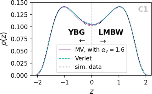
Figure 1
Figure 1. Selection of external potentials. The softened repulsive hard-wall potential 26 is used to test the contact theorem. Its exponential tail is shown in panel A. The soft parts of both confining external potentials 27 and 28 are shown in panel B.
High Resolution Image
Download MS PowerPoint Slide
Figure 2
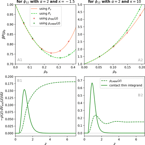
Figure 2. Testing the contact theorem. We consider two types of HCY particles 25, both with α = 2. Column 1, shows results for κ = −1.5 < 0, thus an attractive tail. Column 2, shows results for particles with a repulsive tail, with κ = 10 > 0. In panels A, we show reduced pressure curves calculated using both the virial 3 and compressibility 7 equations of state, given by the solid orange and dashed lime green curves, respectively. The red circles show the results obtained via eq 24, when the input density profile is generated by the YBG eq 17. The green circles show the same, when the input density profile is generated by the LMBW eq 20. In panels B, we show the contact theorem integrand as solid green lines and the density profile generated by the LMBW equation as dashed green lines, to illustrate how we obtain the circles shown in panels A.
High Resolution Image
Download MS PowerPoint Slide
Figure 3
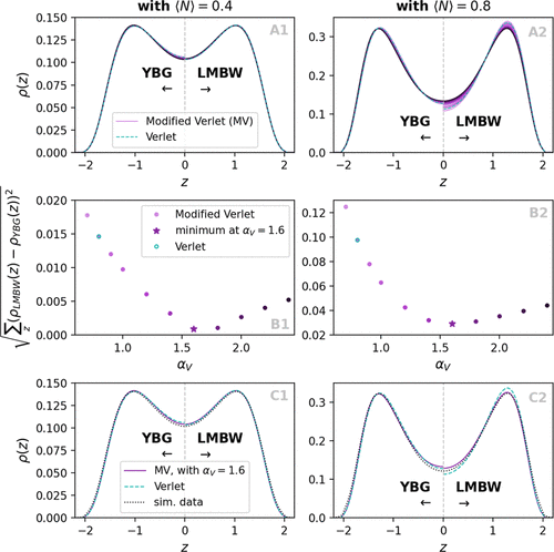
Figure 3. Optimization of the density profiles using the Modified Verlet closure. In panels A we show density profiles calculated using the YBG and LMBW equations for various values of the optimization parameter, α_V. Since the profiles are symmetric about z = 0 we show both YBG and LMBW profiles on the same plot for ease of comparison. The left column of panels concern results for ⟨N⟩ = 0.4, while the right column is for ⟨N⟩ = 0.8. Panels B show the root-mean-square difference between the profiles obtained using the two different routes as a function of α_V. The minimum of both curves is found to be at α_V = 1.6. Panels C show the profiles at this optimal value of α_V and demonstrate the improved structural consistency compared with the standard Verlet closure. We also show simulation data as dotted black curves for comparison.
High Resolution Image
Download MS PowerPoint Slide
Figure 4
Figure 4. Bulk pressure optimization using the Modified Verlet closure. In panel A we show the bulk pressure from the virial 3 and compressibility 7 equations as a function of the bulk density. The dashed sea green lines show the results obtained using the standard Verlet closure, as in Figure 2. Increasing the parameter α_V from 0.8 (the standard Verlet value) to 1.6 leads to a reduction of thermodynamic inconsistency. Virial pressures are shown as solid lime green lines, while the compressibility pressures are shown in orange. In panel B we show only the pressures for the standard Verlet closure and the Modified Verlet closure with the optimized α_V = 1.6. Panels C show zooms of the data from panel B to focus on different density regimes. We added simulation data as dotted black curves to panels B and C for comparison.
High Resolution Image
Download MS PowerPoint Slide
Figure 5
Figure 5. Application of the optimized closure to a harmonic trap. We show density profiles in the external field 28. In panels A the average number of particles per unit length is ⟨N⟩ = 0.8, while in panels B its value is ⟨N⟩ = 1.0. The first column (in sea green) shows results using the standard Verlet closure. The second column (in purple) shows results using the Modified Verlet closure for fixed optimized α_V = 1.6. The density profiles calculated with the LMBW equation are given by solid green lines and the ones calculated with the YBG equation are in dashed red. The simulation data are given by the dotted black curves. It is clear that in both test-cases the Modified Verlet closure with α_V = 1.6 reduces the structural inconsistency in comparison to the results from the standard Verlet closure.
High Resolution Image
Download MS PowerPoint Slide
References
This article references 71 other publications.
1. 1
  Rosenfeld, Y. Free-energy model for the inhomogeneous hard-sphere fluid mixture and density-functional theory of freezing. Phys. Rev. Lett. 1989, 63, 980, DOI: 10.1103/PhysRevLett.63.980
  There is no corresponding record for this reference.
2. 2
  Tarazona, P. Density functional for hard sphere crystals: A fundamental measure approach. Phys. Rev. Lett. 2000, 84, 694, DOI: 10.1103/PhysRevLett.84.694
  There is no corresponding record for this reference.
3. 3
  Roth, R. Fundamental measure theory for hard-sphere mixtures: a review. J. Phys.:Condens. Matter 2010, 22, 063102, DOI: 10.1088/0953-8984/22/6/063102
  There is no corresponding record for this reference.
4. 4
  Wittmann, R.; Marechal, M.; Mecke, K. Fundamental mixed measure theory for non-spherical colloids. Europhys. Lett. 2015, 109, 26003, DOI: 10.1209/0295-5075/109/26003
  There is no corresponding record for this reference.
5. 5
  Cuesta, J. A. Fluid mixtures of parallel hard cubes. Phys. Rev. Lett. 1996, 76, 3742, DOI: 10.1103/PhysRevLett.76.3742
  There is no corresponding record for this reference.
6. 6
  Roth, R.; Mecke, K.; Oettel, M. Communication: Fundamental measure theory for hard disks: Fluid and solid. J. Chem. Phys. 2012, 136, 081101, DOI: 10.1063/1.3687921
  There is no corresponding record for this reference.
7. 7
  Barker, J. A.; Henderson, D. What is liquid? understanding the states of matter. Rev. Mod. Phys. 1976, 48, 587, DOI: 10.1103/RevModPhys.48.587
  There is no corresponding record for this reference.
8. 8
  Evans, R. The nature of the liquid-vapour interface and other topics in the statistical mechanics of non-uniform, classical fluids. Adv. Phys. 1979, 28, 143, DOI: 10.1080/00018737900101365
  There is no corresponding record for this reference.
9. 9
  Evans, R. In Ch. 3 in Fundamentals of Inhomogeneous Fluids; Henderson, D., Ed.; Marcel Dekker: New York, 1992.
  There is no corresponding record for this reference.
10. 10
  Rosenfeld, Y. Free energy model for inhomogeneous fluid mixtures: Yukawa-charged hard spheres, general interactions, and plasmas. J. Chem. Phys. 1993, 98, 8126, DOI: 10.1063/1.464569
  There is no corresponding record for this reference.
11. 11
  Oettel, M. Integral equations for simple fluids in a general reference functional approach. J. Phys.:Condens. Matter 2005, 17, 429, DOI: 10.1088/0953-8984/17/3/003
  There is no corresponding record for this reference.
12. 12
  Tschopp, S. M.; Vuijk, H. D.; Sharma, A.; Brader, J. M. Mean-field theory of inhomogeneous fluids. Phys. Rev. E 2020, 102, 042140, DOI: 10.1103/PhysRevE.102.042140
  There is no corresponding record for this reference.
13. 13
  Dijkman, J.; Dijkstra, M.; van Roij, R.; Welling, M.; van de Meent, J.-W.; Ensing, B. Learning neural free-energy functionals with pair-correlation matching. Phys. Rev. Lett. 2025, 134, 056103, DOI: 10.1103/PhysRevLett.134.056103
  There is no corresponding record for this reference.
14. 14
  Sammüller, F.; Hermann, S.; de las Heras, D.; Schmidt, M. Neural functional theory for inhomogeneous fluids: Fundamentals and applications. Proc. Natl. Acad. Sci. U.S.A. 2023, 120, e2312484120 DOI: 10.1073/pnas.2312484120
  There is no corresponding record for this reference.
15. 15
  Sammüller, F.; Hermann, S.; Schmidt, M. Why neural functionals suit statistical mechanics. J. Phys.: Condens. Matter 2024, 36, 243002, DOI: 10.1088/1361-648X/ad326f
  There is no corresponding record for this reference.
16. 16
  ter Rele, T.; Campos-Villalobos, G.; van Roij, R.; Dijkstra, M. Machine learning many-body potentials for charged colloids in primitive 1:1 electrolytes. arXiv 2025, arXiv.2507.12934, DOI: 10.48550/arXiv.2507.12934
  There is no corresponding record for this reference.
17. 17
  Simon, A.; Weimar, J.; Martius, G.; Oettel, M. Machine learning of a density functional for anisotropic patchy particles. J. Chem. Theory Comput. 2024, 20, 1062, DOI: 10.1021/acs.jctc.3c01238
  There is no corresponding record for this reference.
18. 18
  Simon, A.; Belloni, L.; Borgis, D.; Oettel, M. The orientational structure of a model patchy particle fluid: Simulations, integral equations, density functional theory, and machine learning. J. Chem. Phys. 2025, 162, 034503, DOI: 10.1063/5.0248694
  There is no corresponding record for this reference.
19. 19
  Simon, A.; Oettel, M. Machine learning approaches to classical density functional theory. arXiv 2024, arXiv.2406.07345, DOI: 10.48550/arXiv.2406.07345
  There is no corresponding record for this reference.
20. 20
  Henderson, D. In Ch. 4 in Fundamentals of Inhomogeneous Fluids; Henderson, D., Ed.; Marcel Dekker: New York, 1992.
  There is no corresponding record for this reference.
21. 21
  Tschopp, S. M.; Vahid, H.; Sharma, A.; Brader, J. M. Combining integral equation closures with force density functional theory for the study of inhomogeneous fluids. Soft Matter 2025, 21, 2633, DOI: 10.1039/D4SM01262C
  There is no corresponding record for this reference.
22. 22
  Hansen, J.-P.; McDonald, I. R. Theory of Simple Liquids; Elsevier Science: Amsterdam, 2006.
  There is no corresponding record for this reference.
23. 23
  McQuarrie, D. A. Statistical Mechanics; University Science Books: CA, 2000.
  There is no corresponding record for this reference.
24. 24
  Caccamo, C. Integral equation theory description of phase equilibria in classical fluids. Phys. Rep. 1996, 274, 1, DOI: 10.1016/0370-1573(96)00011-7
  There is no corresponding record for this reference.
25. 25
  Pihlajamaa, I.; Janssen, L. M. C. Comparison of integral equation theories of the liquid state. Phys. Rev. E 2024, 110, 044608, DOI: 10.1103/PhysRevE.110.044608
  There is no corresponding record for this reference.
26. 26
  Bomont, J.-M. Recent advances in the field of integral equation theories: bridge functions and applications to classical fluids. Adv. Chem. Phys. 2008, 139, 1– 84, DOI: 10.1002/9780470259498.ch1
  There is no corresponding record for this reference.
27. 27
  Waisman, E. The radial distribution function for a fluid of hard spheres at high densities. Mol. Phys. 1973, 25, 45, DOI: 10.1080/00268977300100061
  There is no corresponding record for this reference.
28. 28
  Ho/ye, J. S.; Stell, G. Thermodynamics of the msa for simple fluids. J. Chem. Phys. 1977, 67, 439– 445, DOI: 10.1063/1.434887
  There is no corresponding record for this reference.
29. 29
  Rosenfeld, Y.; Ashcroft, N. W. Theory of simple classical fluids: Universality in the short-range structure. Phys. Rev. A 1979, 20, 1208, DOI: 10.1103/PhysRevA.20.1208
  There is no corresponding record for this reference.
30. 30
  Verlet, L. Integral equations for classical fluids. Mol. Phys. 1980, 41, 183, DOI: 10.1080/00268978000102671
  There is no corresponding record for this reference.
31. 31
  Rogers, F. J.; Young, D. A. New, thermodynamically consistent, integral equation for simple fluids. Phys. Rev. A 1984, 30, 999, DOI: 10.1103/PhysRevA.30.999
  There is no corresponding record for this reference.
32. 32
  Zerah, G.; Hansen, J.-P. Self-consistent integral equations for fluid pair distribution functions: Another attempt. J. Chem. Phys. 1986, 84, 2336, DOI: 10.1063/1.450397
  There is no corresponding record for this reference.
33. 33
  Ballone, P.; Pastore, G.; Gazzillo, D. Additive and non-additive hard sphere mixtures. Mol. Phys. 1986, 59, 275, DOI: 10.1080/00268978600102071
  There is no corresponding record for this reference.
34. 34
  Pini, D.; Stell, G.; Wilding, N. A liquid-state theory that remains successful in the critical region. Mol. Phys. 1998, 95, 483, DOI: 10.1080/00268979809483183
  There is no corresponding record for this reference.
35. 35
  Pini, D.; Stell, G.; Høye, J. Self-consistent approximation for fluids and lattice gases. Int. J. Thermophys. 1998, 19, 1029, DOI: 10.1023/A:1022673222199
  There is no corresponding record for this reference.
36. 36
  Caccamo, C.; Pellicane, G.; Costa, D.; Pini, D.; Stell, G. Thermodynamically self-consistent theories of fluids interacting through short-range forces. Phys. Rev. E 1999, 60, 5533, DOI: 10.1103/PhysRevE.60.5533
  There is no corresponding record for this reference.
37. 37
  Duh, D.; Haymet, A. D. J. Integral equation theory for uncharged liquids: The Lennard-Jones fluid and the bridge function. J. Chem. Phys. 1995, 103, 2625, DOI: 10.1063/1.470724
  There is no corresponding record for this reference.
38. 38
  Duh, D.; Henderson, D. Integral equation theory for Lennard-Jones fluids: The bridge function and applications to pure fluids and mixtures. J. Chem. Phys. 1996, 104, 6742, DOI: 10.1063/1.471391
  There is no corresponding record for this reference.
39. 39
  Parola, A.; Reatto, L. Liquid state theories and critical phenomena. Adv. Phys. 1995, 44, 211, DOI: 10.1080/00018739500101536
  There is no corresponding record for this reference.
40. 40
  Parola, A.; Pini, D.; Reatto, L. The smooth cut-off hierarchical reference theory of fluids. Mol. Phys. 2009, 107, 503, DOI: 10.1080/00268970902873547
  There is no corresponding record for this reference.
41. 41
  Caillol, J.-M. Link between the hierarchical reference theory of liquids and a new version of the non-perturbative renormalization group in statistical field theory. Mol. Phys. 2011, 109, 2813, DOI: 10.1080/00268976.2011.621455
  There is no corresponding record for this reference.
42. 42
  Parola, A.; Reatto, L. Recent developments of the hierarchical reference theory of fluids and its relation to the renormalization group. Mol. Phys. 2012, 110, 2859, DOI: 10.1080/00268976.2012.666573
  There is no corresponding record for this reference.
43. 43
  Lee, L. L. An accurate integral equation theory for hard spheres: Role of the zero-separation theorems in the closure relation. J. Chem. Phys. 1995, 103, 9388, DOI: 10.1063/1.469998
  There is no corresponding record for this reference.
44. 44
  Lee, L. L. The potential distribution-based closures to the integral equations for liquid structure: The Lennard-Jones fluid. J. Chem. Phys. 1997, 107, 7360, DOI: 10.1063/1.474974
  There is no corresponding record for this reference.
45. 45
  Yuste, S. B.; Santos, A. Radial distribution function for hard spheres. Phys. Rev. A 1991, 43, 5418, DOI: 10.1103/PhysRevA.43.5418
  There is no corresponding record for this reference.
46. 46
  Yuste, S. B.; Santos, A.; López de Haro, M. Structure of multi-component hard-sphere mixtures. J. Chem. Phys. 1998, 108, 3683, DOI: 10.1063/1.475762
  There is no corresponding record for this reference.
47. 47
  Choudhury, N.; Ghosh, S. K. Integral equation theory of Lennard-Jones fluids: A modified Verlet bridge function approach. J. Chem. Phys. 2002, 116, 8517, DOI: 10.1063/1.1467894
  There is no corresponding record for this reference.
48. 48
  Bomont, J. M.; Bretonnet, J. L. A self-consistent integral equation: Bridge function and thermodynamic properties for the Lennard-Jones fluid. J. Chem. Phys. 2003, 119, 2188, DOI: 10.1063/1.1583675
  There is no corresponding record for this reference.
49. 49
  Carbajal-Tinoco, M. D. Thermodynamically consistent integral equation for soft repulsive spheres. J. Chem. Phys. 2008, 128, 184507, DOI: 10.1063/1.2918495
  There is no corresponding record for this reference.
50. 50
  Rowlinson, J. S.; Widom, B. Molecular Theory of Capillarity; Dover: New York, 2003.
  There is no corresponding record for this reference.
51. 51
  Henderson, J. In Ch. 2 in Fundamentals of Inhomogeneous Fluids; Henderson, D., Ed.; Marcel Dekker: New York, 1992.
  There is no corresponding record for this reference.
52. 52
  Attard, P. Thermodynamics and Statistical Mechanics; Academic Press: Amsterdam, 2002.
  There is no corresponding record for this reference.
53. 53
  Yvon, J. La théorie statistique des fluides et l’équation d’état; Hermann: Paris, 1935.
  There is no corresponding record for this reference.
54. 54
  Born, M.; Green, H. S. A general kinetic theory of liquids I. the molecular distribution functions. Proc. R. Soc. A 1946, 188, 10, DOI: 10.1098/rspa.1946.0093
  There is no corresponding record for this reference.
55. 55
  Lovett, R. A.; Mou, C. Y.; Buff, F. P. The structure of the liquid–vapor interface. J. Chem. Phys. 1976, 65, 570, DOI: 10.1063/1.433110
  There is no corresponding record for this reference.
56. 56
  Wertheim, M. S. Correlations in the liquid–vapor interface. J. Chem. Phys. 1976, 65, 2377, DOI: 10.1063/1.433352
  There is no corresponding record for this reference.
57. 57
  Lovett, R. A.; Buff, F. P. Examples of the construction of integral equations in equilibrium statistical mechanics from invariance principles. Phys. A 1991, 172, 147, DOI: 10.1016/0378-4371(91)90317-6
  There is no corresponding record for this reference.
58. 58
  Baus, M.; Lovett, R. A. A direct derivation of the profile equations of Buff-Lovett-Mou-Wertheim from the Born-Green-Yvon equations for a non-uniform equilibrium fluid. Phys. A 1992, 181, 329, DOI: 10.1016/0378-4371(92)90092-5
  There is no corresponding record for this reference.
59. 59
  Omelyan, I.; Hirata, F.; Kovalenko, A. Criticality of a liquid–vapor interface from an inhomogeneous integral equation theory. Phys. Chem. Chem. Phys. 2005, 7, 4132, DOI: 10.1039/b507761c
  There is no corresponding record for this reference.
60. 60
  Brader, J. M. Structural precursor to freezing: an integral equation study. J. Chem. Phys. 2008, 128, 104503, DOI: 10.1063/1.2889926
  There is no corresponding record for this reference.
61. 61
  Nygård, K.; Sarman, S.; Kjellander, R. Local order variations in confined hard-sphere fluids. J. Chem. Phys. 2013, 139, 164701, DOI: 10.1063/1.4825176
  There is no corresponding record for this reference.
62. 62
  Nygård, K.; Sarman, S.; Hyltegren, K.; Chodankar, S.; Perret, E.; Buitenhuis, J.; van der Veen, J. F.; Kjellander, R. Density fluctuations of hard-sphere fluids in narrow confinement. Phys. Rev. X 2016, 6, 011014, DOI: 10.1103/PhysRevX.6.011014
  There is no corresponding record for this reference.
63. 63
  Attard, P. Spherically inhomogeneous fluids. i. percus–yevick hard spheres: Osmotic coefficients and triplet correlations. J. Chem. Phys. 1989, 91, 3072, DOI: 10.1063/1.456930
  There is no corresponding record for this reference.
64. 64
  Attard, P. Spherically inhomogeneous fluids. ii. hard-sphere solute in a hard-sphere solvent. J. Chem. Phys. 1989, 91, 3083, DOI: 10.1063/1.456931
  There is no corresponding record for this reference.
65. 65
  Kjellander, R.; Sarman, S. On the statistical mechanics of inhomogeneous fluids in narrow slits. an application to a hard-sphere fluid between hard walls. Chem. Phys. Lett. 1988, 149, 102, DOI: 10.1016/0009-2614(88)80357-9
  There is no corresponding record for this reference.
66. 66
  Tschopp, S. M.; Sammüller, F.; Hermann, S.; Schmidt, M.; Brader, J. M. Force density functional theory in- and out-of-equilibrium. Phys. Rev. E 2022, 106, 014115, DOI: 10.1103/PhysRevE.106.014115
  There is no corresponding record for this reference.
67. 67
  Yvon, J. Note sur un calcul de perturbation en mécanique statistique. Il Nuovo Cimento 1958, 9, 144, DOI: 10.1007/BF02824240
  There is no corresponding record for this reference.
68. 68
  Evans, R.; Dolny, K. Density Functional Theory for Inhomogeneous Fluids I: Simple Fluids in Equilibrium, Lecture notes in physics; University of Bristol, 2009.
  There is no corresponding record for this reference.
69. 69
  Lado, F. Numerical fourier transforms in one, two, and three dimensions for liquid state calculations. J. Comput. Phys. 1971, 8, 417, DOI: 10.1016/0021-9991(71)90021-0
  There is no corresponding record for this reference.
70. 70
  Thompson, A. P.; Aktulga, H. M.; Berger, R.; Bolintineanu, D. S.; Brown, W. M.; Crozier, P. S.; in ’t Veld, P. J.; Kohlmeyer, A.; Moore, S. G.; Nguyen, T. D.; Shan, R.; Stevens, M. J.; Tranchida, J.; Trott, C.; Plimpton, S. J. LAMMPS - a flexible simulation tool for particle-based materials modeling at the atomic, meso, and continuum scales. Comput. Phys. Commun. 2022, 271, 108171, DOI: 10.1016/j.cpc.2021.108171
  There is no corresponding record for this reference.
71. 71
  Tschopp, S. M.; Brader, J. M. First-principles superadiabatic theory for the dynamics of inhomogeneous fluids. J. Chem. Phys. 2022, 157, 234108, DOI: 10.1063/5.0131441
  There is no corresponding record for this reference.

Routes to the Density Profile and Structural InconsistencyClick to copy article linkArticle link copied!

The Journal of Physical Chemistry B

Abstract

Special Issue

1. Introduction

2. Methods

2.1. Bulk Fluids

2.1.1. The Bulk Ornstein–Zernike Equation

2.1.2. Two Routes to Calculate the Pressure

2.1.2.1. The Virial Route

2.1.2.2. The Compressibility Route

2.2. Inhomogeneous Fluids

2.2.1. The Inhomogeneous Ornstein–Zernike Equation

2.2.2. Two Routes to the One-Body Density

2.2.2.1. The Yvon–Born–Green Equation

2.2.2.2. The Lovett–Mou–Buff–Wertheim Equation

2.2.3. Closure Relation Approximations

2.2.4. Wall Contact Theorem

2.3. Numerical Implementation

2.3.1. System of Interest: Specification of the Interparticle and External Potentials

2.3.1.1. Choice of the Interparticle Pair Potential

2.3.1.2. Choice of External Potentials

Figure 1

2.3.2. Obtaining the Inhomogeneous Density Profiles

2.3.2.1. YBG and LMBW DFT in Two-Dimensional Planar Geometry

2.3.2.2. Accounting for Discontinuities

2.3.2.3. The Inhomogeneous OZ Equation in Two-Dimensional Planar Geometry

2.3.3. Generating Simulation Data for Comparison

3. Results

3.1. Contact Theorem

Figure 2

3.2. Optimization by Enforcing Structural Consistency

3.2.1. Packed System

Figure 3

3.2.2. Pressure Curves

Figure 4

3.3. Test on a Different External Potential

Figure 5

4. Discussion & Conclusions

Author Information

Appendix A

Detailed Calculations to Account for Discontinuities

Appendix B

Details on the Simulation Data Curves

Packed System

Pressure Curve

Test on a Different External Potential

References

Cited By

The Journal of Physical Chemistry B

Article Views

Altmetric

Citations

Recommended Articles

Abstract

Figure 1

Figure 2

Figure 3

Figure 4

Figure 5

References

Routes to the Density Profile and Structural Inconsistency
Click to copy article linkArticle link copied!